A Survey on Discrete Laplacians
for General
Polygonal Meshes

Problem Setting
Solve PDEs on surface meshes and volume meshes
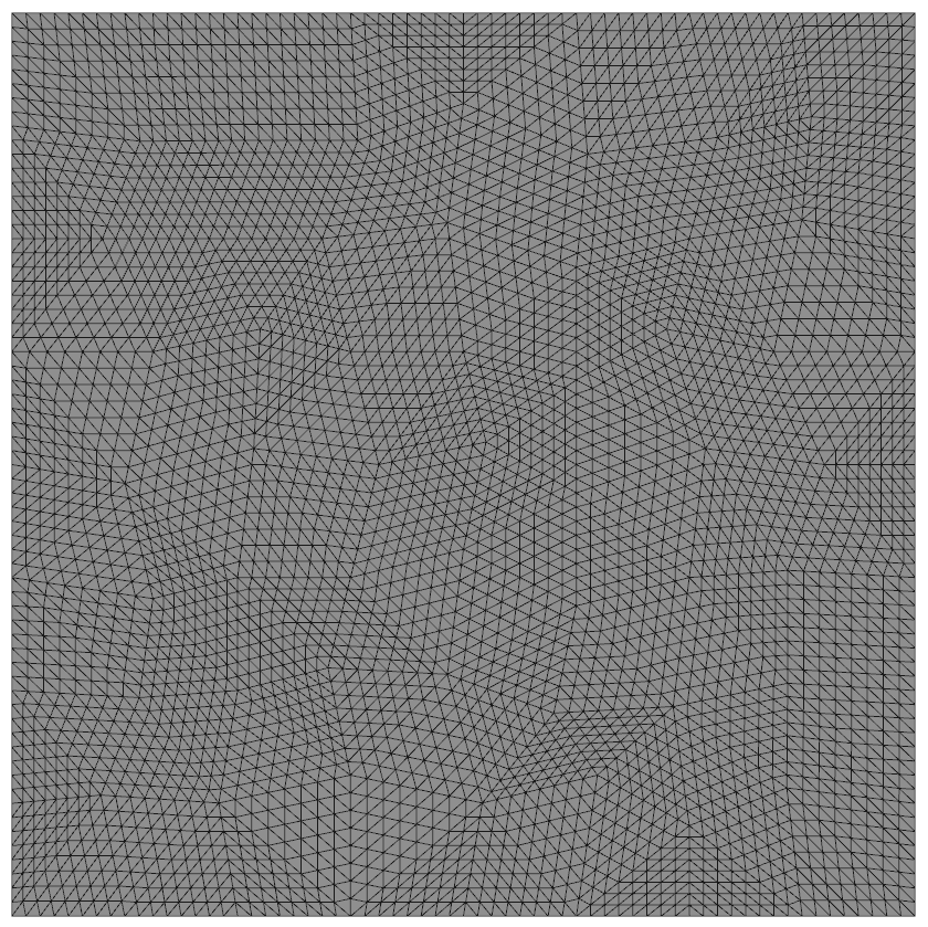
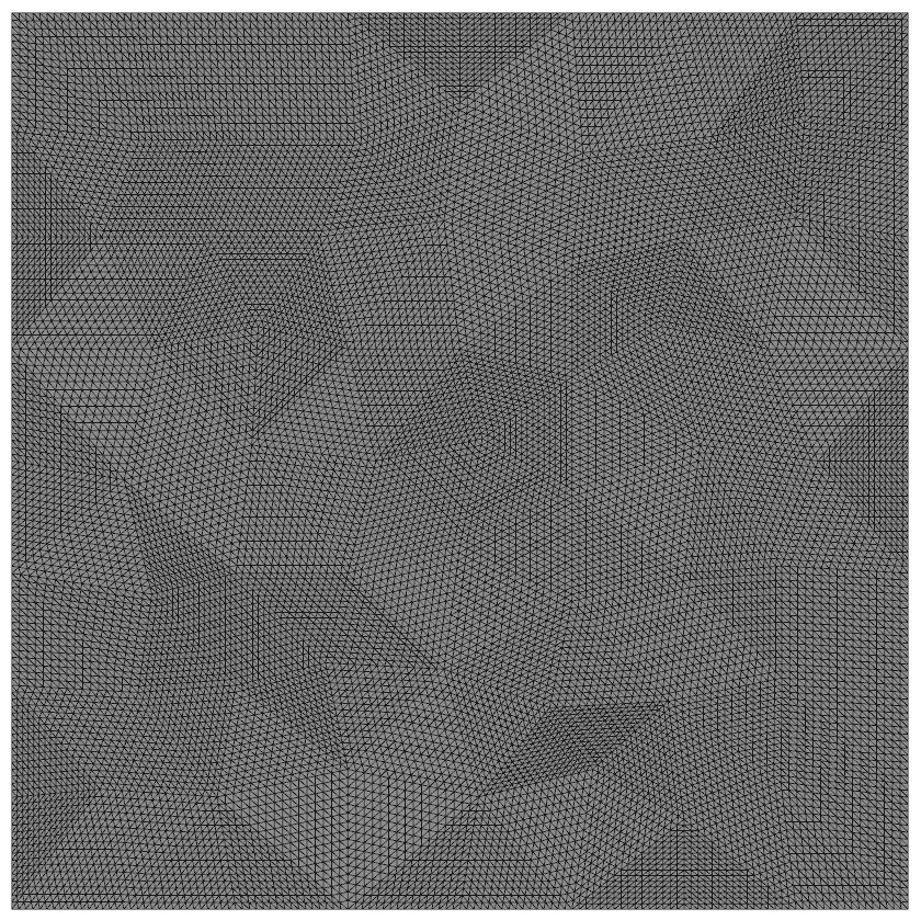
 Surface triangle mesh
  Volume tetrahedral mesh
Discrete Laplacian has various applications
- Mean Curvature
- Smoothing & Fairing
- Parameterization
- Deformation
- Geodesics Distances
- …

Discrete Laplacians for Polygonal/Polyhedral Meshes
Surface Meshes: Triangles Polygons Volume Meshes: Tetrahedra Polyhedra
Flatland

Discrete Laplacians for Polygonal Meshes
Surface Meshes: Triangles Polygons Volume Meshes: Tetrahedra Polyhedra
Triangulate the Polygons?


Triangle Meshes

- Connectivity / Topology
- Vertices \(\mathcal{V} = \{ v_1, \dots, v_n \}\)
- Edges \(\mathcal{E} = \{ e_1, \dots, e_k \}\), \(e_i \in \mathcal{V} \times \mathcal{V}\)
- Faces \(\mathcal{F} = \{ f_1, \dots, f_m \}\), \(f_i \in \mathcal{V} \times \mathcal{V} \times \mathcal{V}\)

- Geometry
- Vertex positions \(\{ \vec{x}_1, \dots, \vec{x}_n \}\), \(\vec{x}_i \in \R^3\)
Functions on Triangle Meshes
- Define a piecewise linear function on a triangle mesh as \[f(\vec{x}) = \sum_{i \in \set{V}} f_i \varphi_i(\vec{x})\]
- Assign function values \(f_i\) to vertices \(v_i\) with positions \(\vec{x}_i\)
- Assign linear “hat” basis functions \(\varphi_i(\vec{x})\) to vertices \(v_i\)
- Equivalent to barycentric interpolation of \(f_i\) within triangles

Laplace Matrix & Mass Matrix
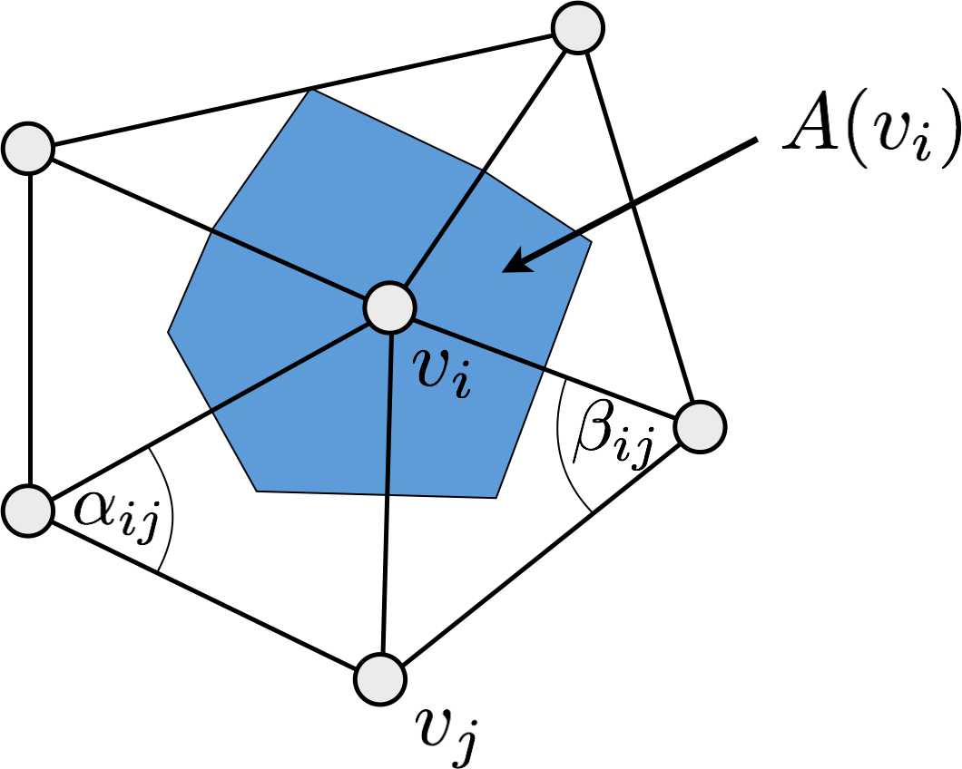
\[ \small \begin{eqnarray*} \mat{L}_{ij} &=& -\int \grad \varphi_i \cdot \grad \varphi_j &=& \begin{cases} \frac{\cot\alpha_{ij}+\cot\beta_{ij}}{2} & \text{if } j\in\set{N}\of{i} \,, \\[0.5em] \displaystyle -\sum_{k\in\set{N}\of{i}} \mat{L}_{ik} & \text{if } j=i \,, \\[0.3em] 0 & \text{otherwise}. \end{cases} \\[1em] \mat{M}_{ij} &=& \int \varphi_i \, \varphi_j &=& \begin{cases} \frac{\abs{t_{ijk}} + \abs{t_{jih}}}{12} & \text{if } j\in\set{N}\of{i}\,, \\[0.5em] \displaystyle \sum_{k\in\set{N}\of{i}} \mat{M}_{ik} & \text{if }j=i \,,\\[0.3em] 0 & \text{otherwise}. \end{cases} \end{eqnarray*} \]
Local to Global Assembly


Properties
- Symmetry
- Locality
- Linear precision
- Negative semi-definiteness
- Null property
- Positive weights

Poisson System on 2D Triangle Meshes
Generalized Barycentric Coordinates
- Wachspress Coordinates
- Wachspress, Warren
- Mean Value Coordinates
- Floater, Hormann, Ju, Wicke
- Maximum Entropy Coordinates
- Sukumar, Hormann
- Harmonic Coordinates
- Joshi, Martin
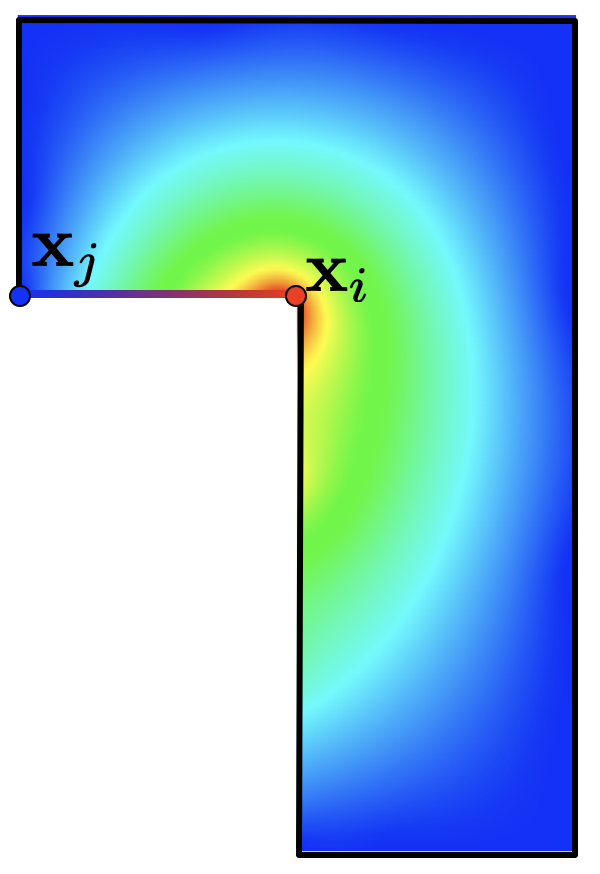
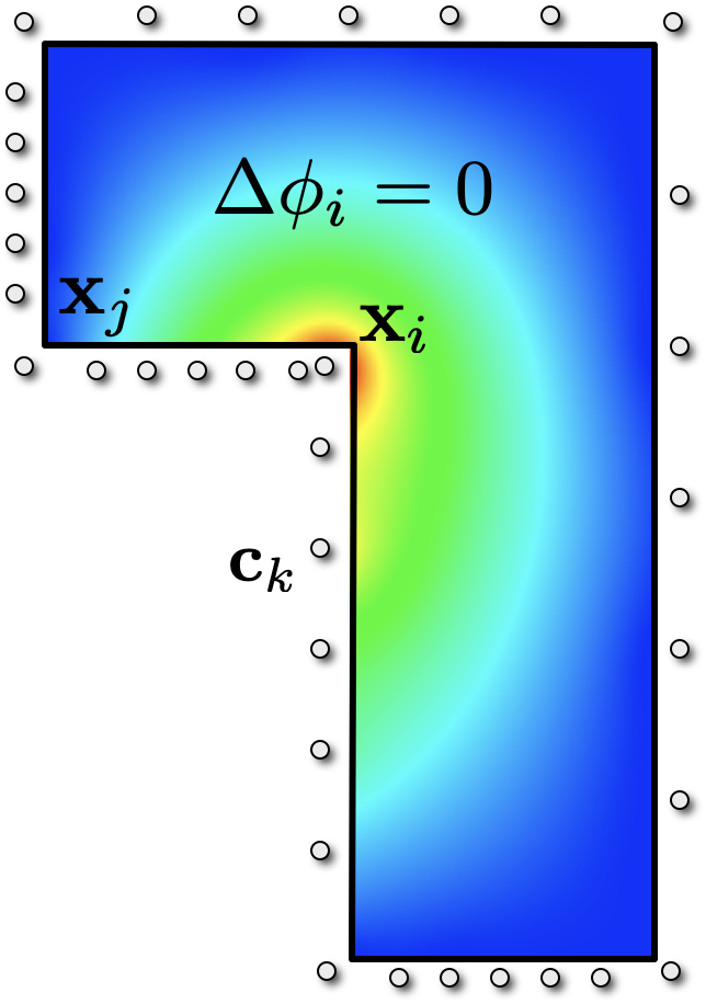
Harmonic Coordinates
- Definition
- Interpolate nodal data: \(\varphi_i(\vec{x}_j) = \delta_{ij}\)
- Linear (=harmonic) on edges
- Harmonic in interior: \(\laplace\varphi_i = 0\)
- Computation
- Method of fundamental solutions
- Approximate shape functions \(\varphi_i\) by RBFs \(\psi_k\) \[\varphi_i(\vec{x}) = \sum_k w_k \, \psi_k\of{\vec{x}} + \pi_1\of{\vec{x}}\]
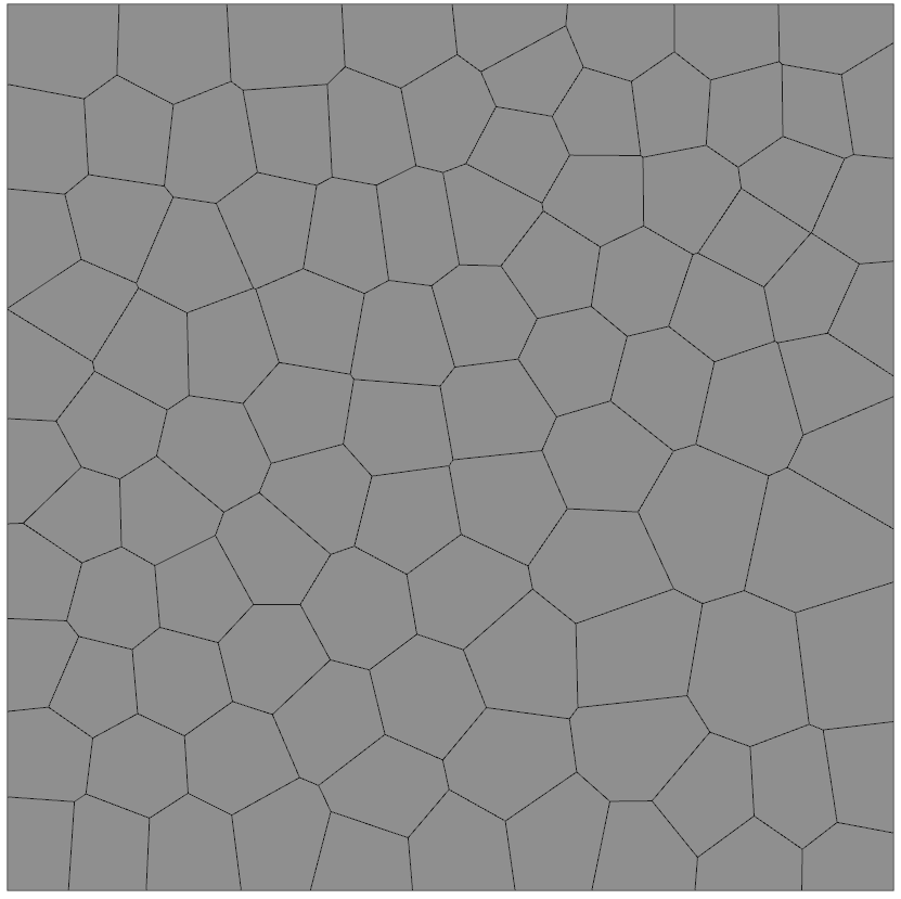
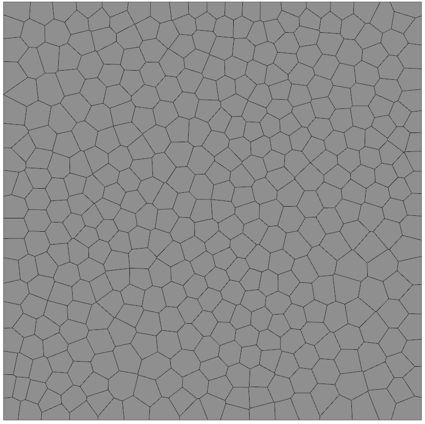
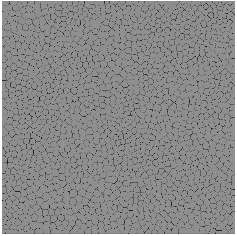
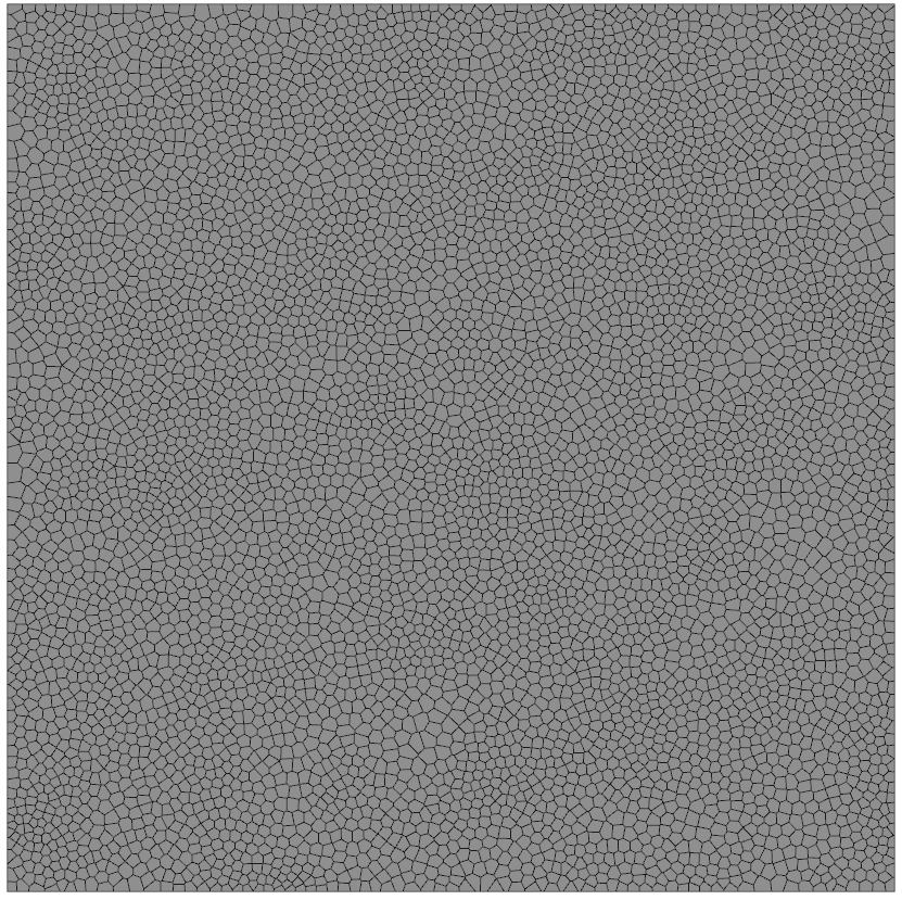
Poisson System on 2D Voronoi Meshes
DEC Polygon Laplacians
- Generalize DEC to non-planar polygons
- Both have to tune a hyper-parameter \(\lambda\) \[\small \laplace \vec{u} \;\approx\; \mat{M}_0^{-1} \underbrace{\mat{d}\T \mat{M}_1 \mat{d}}_{\mat{L}} \, \vec{u}\]
- Inner product matrix \(\mat{M}_1\) has to be positive definite
- Regularization fills up the kernel 👍
- Regularization affects the results 👎
\(k\)-Forms
- Function that takes in \(k\)-simplex and assigns integrated value at output
- Values stored at each element of the mesh
- 0-simplex: Vertices

\(k\)-Forms
- Function that takes in \(k\)-simplex and assigns integrated value at output
- Values stored at each element of the mesh
- 0-simplex: Vertices
- 1-simplex: Edges

\(k\)-Forms
- Function that takes in \(k\)-simplex and assigns integrated value at output
- Values stored at each element of the mesh
- 0-simplex: Vertices
- 1-simplex: Edges
- 2-simplex: Faces

\(k\)-Forms
- Function that takes in \(k\)-simplex and assigns integrated value at output
- Values stored at each element of the mesh
- 0-simplex: Vertices
- 1-simplex: Edges
- 2-simplex: Faces
- Inner product matrix \(\mat{M}_k\) defines a dot product \[ \left\langle \vec{u}, \vec{v} \right\rangle := \vec{u}\tp \mat{M}_k \vec{v} \]
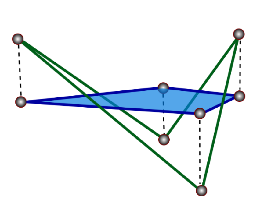
Strategy I: Maximum Orthogonal Projection

Inner Product Matrix
- \(\mat{B}_f = (\vec{b}_1,\dots,\vec{b}_{n_f})^{\mathsf{T}} \in \R^{n_f \times 3}\)
- Rows are barycenters \(\vec{b}_i = \frac{1}{2}\left(\mat{x}_{i+1}+\vec{x}_i\right)\) of each edge \(\vec{e}_i\).
- $|f| $ is vector area of polygon \(f\)
- Define local inner product matrix for 1-forms
- \(\mat{\tilde{M}}_f = \frac{1}{|f|}\mat{B}_f \mat{B}_f ^{\mathsf{T}}\)
- Encodes the polygon’s geometry
Inner Product Matrix
- Laplace matrix \(\tilde{\mat{L}}_f = \mat{d}_f^{\mathsf{T}} \mat{\tilde{M}}_f \mat{d}_f\)
- Matrix \(\mat{d}_f\) is the difference operator on polygon \(f\)
- Gives gradient of vector area \[ \grad_{\vec{x}_i}\abs{f} = \left(\tilde{\mat{L}}_f \mat{X}_f\right)_i \]
- Connection to cotan formula:
- Derived as the gradient of triangle surface area 👍

On some polygons \(\mat{\tilde{M}}_f\) is only positive semi-definite 😢
Fill up the Kernel
- \(\mat{E}_f = (\vec{e}_1,\dots,\vec{e}_{n_f})^{\mathsf{T}} \in \R^{n_f \times 3}\)
- Rows are edge vectors of polygon \(f\).

- Rows are edge vectors of polygon \(f\).
- \(\mathbf{E}_f\T\) has maximal rank 3
- \(\mat{E}_{\bar{f}} = (\bar{\vec{e}}_1,\dots,\bar{\vec{e}}_{n_f})^{\mathsf{T}} \in \R^{n_f \times 3}\)
- Rows are edge vectors of maximal projection \(\bar{f}\).

- Rows are edge vectors of maximal projection \(\bar{f}\).
- \(\mat{E}\T_{\bar{f}}\) has rank 2 \(\rightarrow\) non-trivial kernel
Virtual Simplicial Refinement


Prolongation Operator
\[ {\Huge \downarrow} \; \mat{P} \]
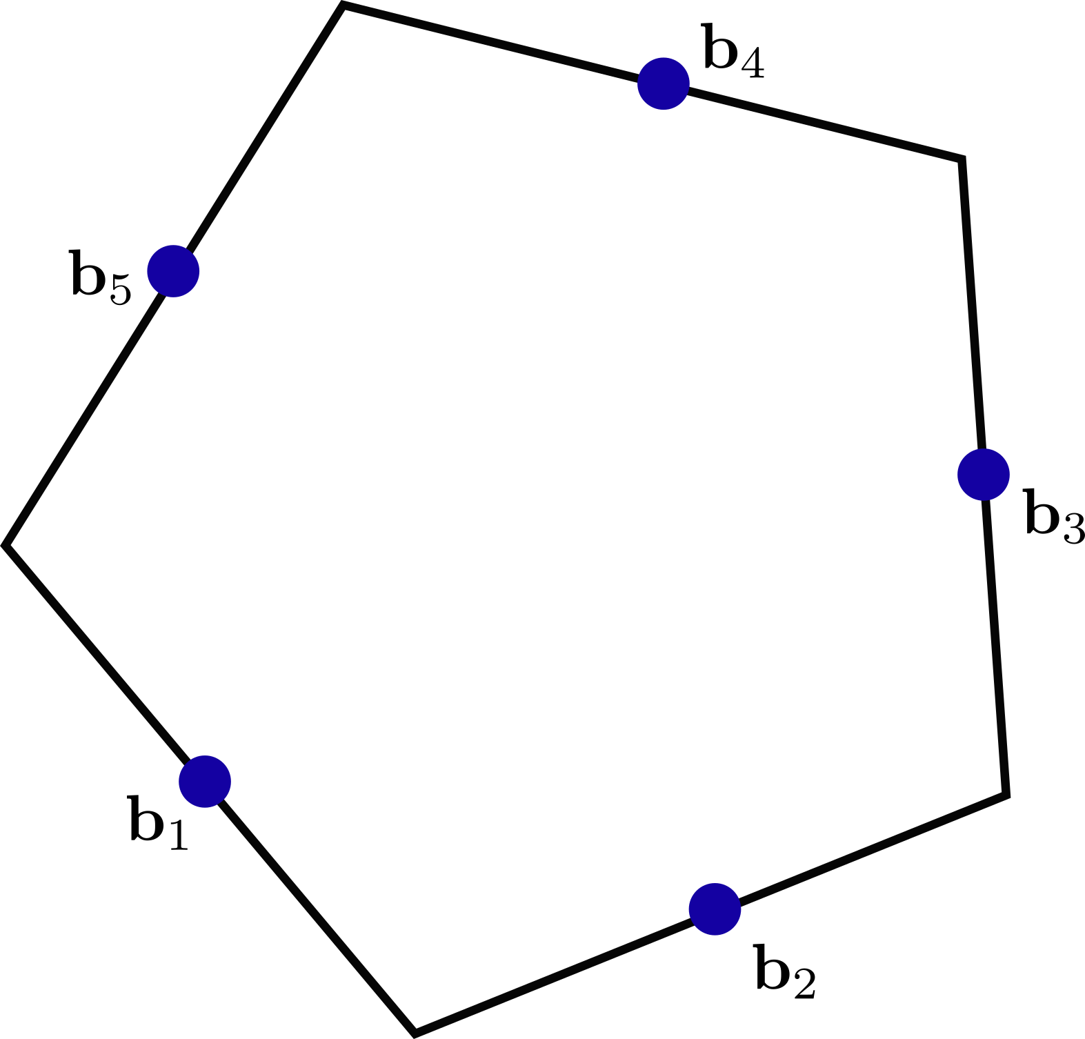
- Insert virtual vertex as affine combination \[ \small \matrix{ \sum_i w_i \vec{x}_{i}\\ \vec{x}_{1}\\ \vec{x}_{2}\\ \vec{x}_{3}\\ \vec{x}_{4}\\ \vec{x}_{5}\\ \vec{x}_{6} } = \underbrace{ \matrix{ w_1 & w_2 & w_3 & w_4 & w_5 & w_6\\ 1 & & & & & \\ & 1 & & & & \\ & & 1 & & & \\ & & & 1 & & \\ & & & & 1 & \\ & & & & & 1 } }_{\mat{P}} \matrix{ \vec{x}_{1}\\ \vec{x}_{2}\\ \vec{x}_{3}\\ \vec{x}_{4}\\ \vec{x}_{5}\\ \vec{x}_{6} } \]
Restriction Operator
\[ {\Huge \uparrow} \; \mat{R} = \mat{P}\T \]
- Redistribute values back to original nodes \[ \mat{R} = \mat{P}\T \]
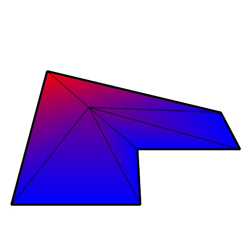
Polygon Shape Functions
\[\downarrow\] \[\downarrow\]
- Insert center vertex through prolongation weights
- Compute standard linear shape functions \(\psi_j(\vec{x})\) on refined polygon
- Coarse shape function for polygon \((\vec{x}_1, \dots, \vec{x}_n)\) with virtual vertex \(\vec{x}_0\) become \[ \varphi_i(\vec{x}) = \psi_i(\vec{x}) + w_i\psi_0(\vec{x}) \,,\quad i \in \{1, \dots, n\} \]
Polygon Shape Functions
- Piecewise linear functions
- Interpolate nodal data: \(\varphi_i\of{\vec{x}_j} = \delta_{ij}\)
- Partition of unity: \(\sum_i \varphi_i\of{\vec{x}} = 1\)
- Barycentric property: \(\sum_i \varphi_i\of{\vec{x}} \vec{x}_i = \vec{x}\)
- \(C^0\) across elements, not \(C^1\) within elements
Choice of Virtual Vertex


Solve linear system for affine prolongation weights 👍
Laplace Matrix & Mass Matrix
- “Sandwiched” Laplace matrix for polygons \[\mat{L} = \mat{P}\T \, \mat{L}^\func{tri} \, \mat{P} \]
- “Sandwiched” mass matrix for polygons \[\mat{M} = \mat{P}\T \, \mat{M}^\func{tri} \, \mat{P} \]
- Laplacian can be factored into divergence and gradient \[ \mat{L} = \underbrace{\mat{P}\T \mat{D}^\func{tri}}_{\mat{D}} \cdot \underbrace{\mat{G}^\func{tri} \mat{P}}_{\mat{G}} \]
Virtual refinement is completely hidden in matrix assembly step!
Discrete Duality Finite Volumes (DDFV)


Quiz
How do we get diamond cells on an arbitrary polygon mesh?
- Subdivide into triangles
- Subdivide into quads
- Connect primal and dual vertices
- Introduce third control mesh


2D DDFV
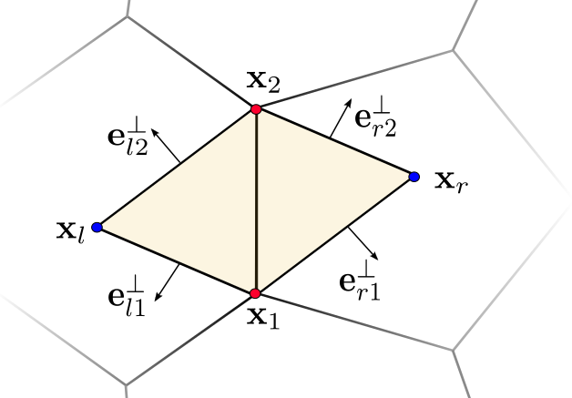
\[ \grad u|_D \;=\; \frac{1}{2 \abs{D}} \sum_{(i,j) \in \partial D} \vec{e}_{ij}^\perp \frac{u_i+u_j}{2} \]
Virtual Dual Vertices
\[\downarrow\] \[\downarrow\]
- Combine ideas from DDFV and virtual refinement
- Use virtual vertices as dual mesh
- Compute DDFV operator on the “virtual diamonds”
- Express diamond in an intrinsic 2D coordinate system
- Restrict values back to the original mesh
Poisson System on 2D Planes

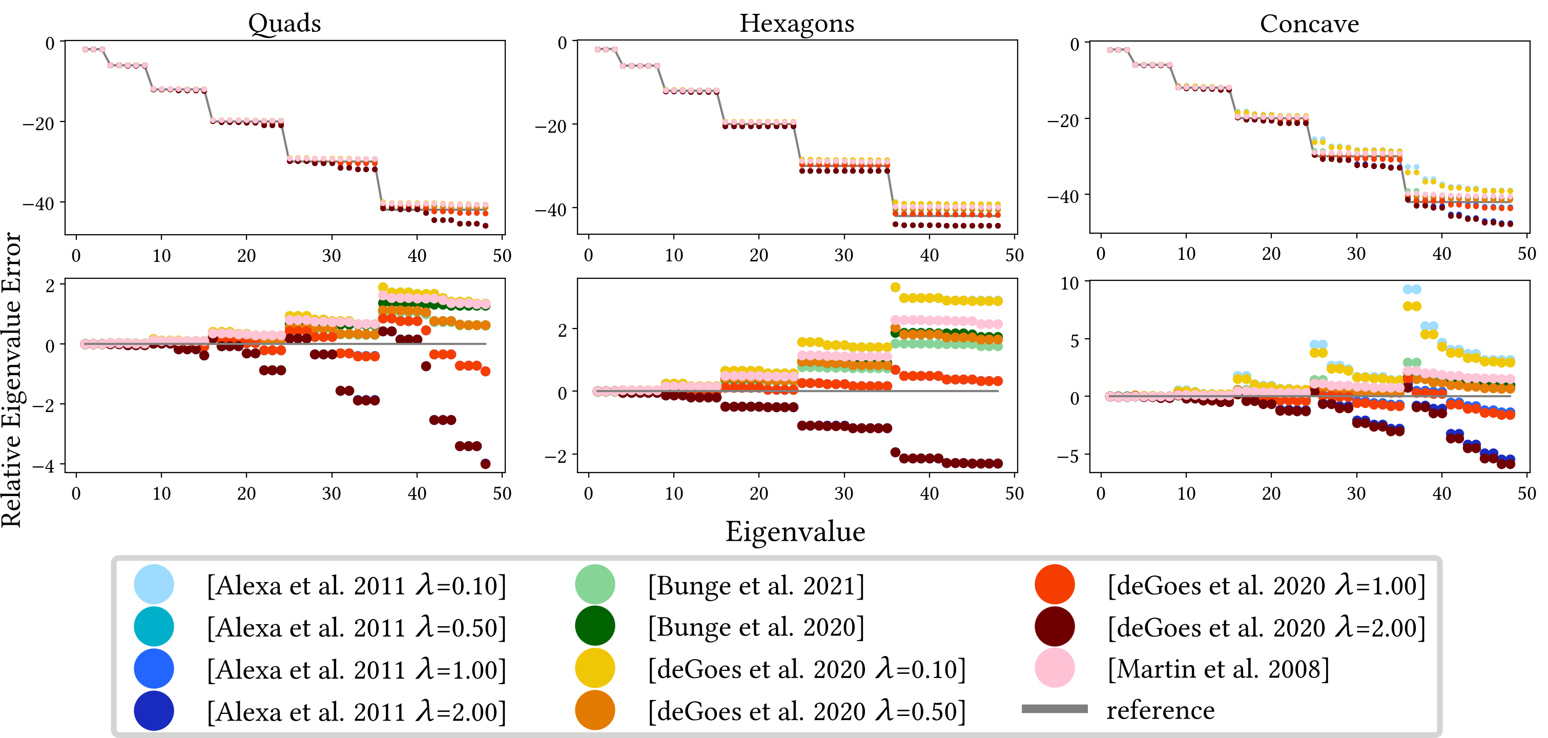
Eigenvalues on Unit Spheres
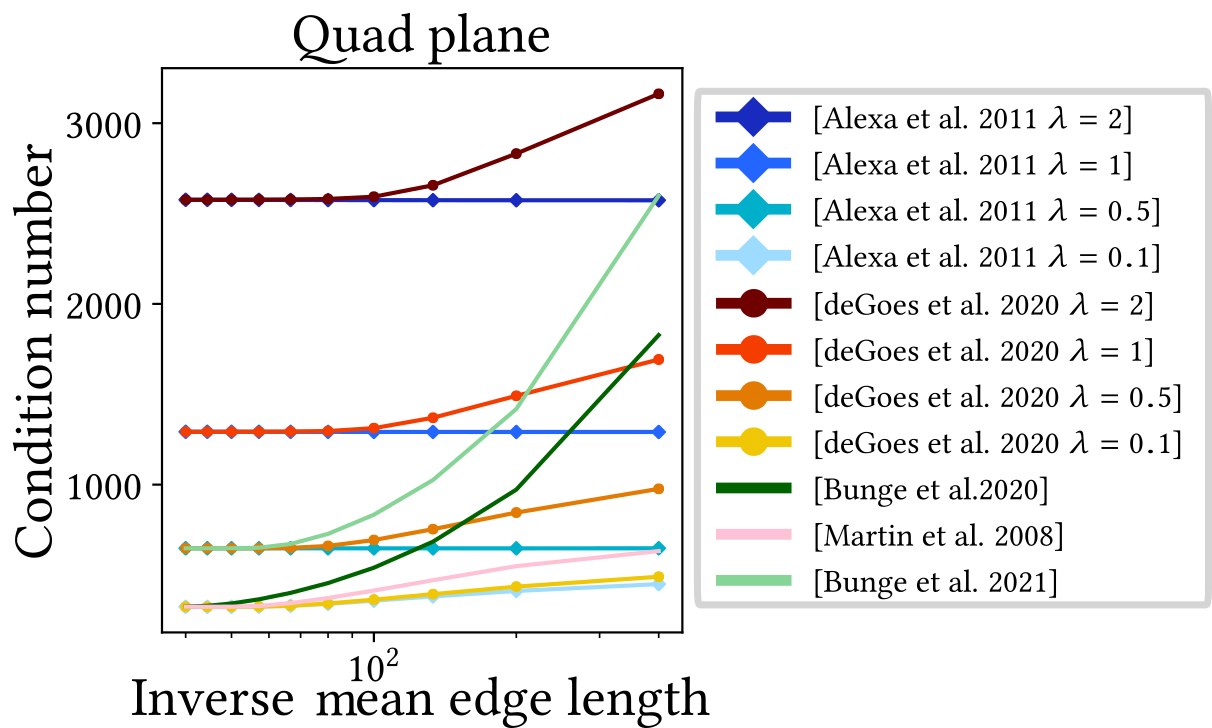
Condition Number
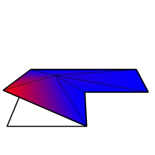
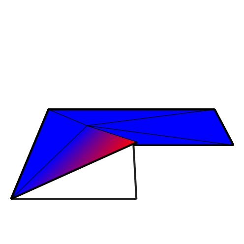
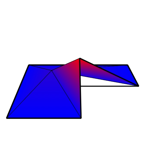
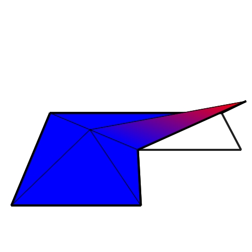
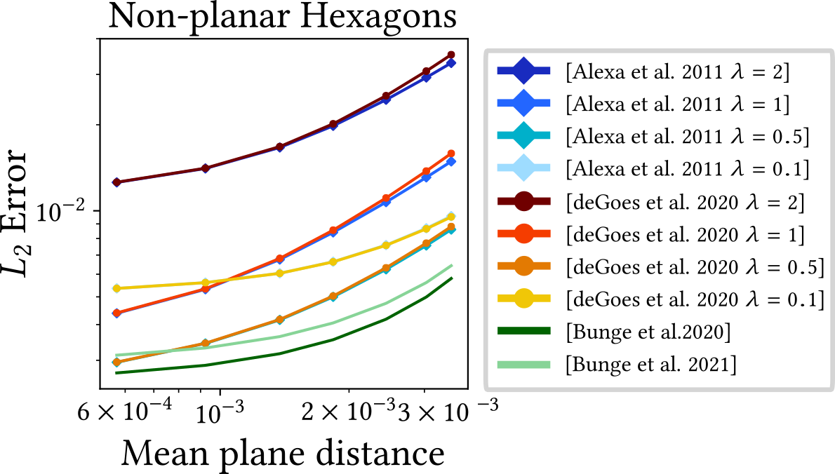
Non-planar Polygons
Computational Performance

Conclusion
- Presented recent progress for Polygon Laplacians
- Discuss individual discretization strategies
- Point out similarities and differences
- Analyze individual strength and weaknesses
- Extensions
- Extension to volume meshes (see STAR (Bunge and Botsch 2023))
- Higher order shape functions (Bunge et al. 2022)

- Acknowledgments
- Collaborators: Marc Alexa, Philipp Herholz, Misha Kazhdan, Olga Sorkine-Hornung
- Code-Checkers: Fernando de Goes, Max Wardetzky